Spectral Feature Fitting (SFF)
SFF measures how well a pixel matches a reference mineral spectrum at its diagnostic absorption features. Rather than comparing the whole curve, it isolates the narrow windows where the mineral absorbs and fits the pixel against the reference there. TerraEye's implementation is multi-range SFF (MrSFF): all of a mineral's absorption windows are fitted together, so a pixel has to match the full set of features, not just one.
It works on continuum-removed spectra, and that is the part that makes it SFF rather than a generic curve comparison. Within each window a straight-line continuum is fitted across the shoulders of the absorption and divided out, in both your pixel and the reference, so what gets compared is the shape and position of the absorption rather than the pixel's overall brightness. The reference feature is then least-squares fitted to yours.
Removing the continuum is why SFF is insensitive to illumination and albedo, and it is the mathematical reason behind the instruction you will see throughout these docs: read the position of a dip, not its depth.
In TerraEye the per-feature fits are combined and scaled so that values run 0 to 1, closer to 1 being a better fit.
Requires hyperspectral data: EMIT, EnMAP or PRISMA. Fitting an individual absorption feature needs contiguous narrow bands, which a multispectral sensor does not have. Note that EMIT only covers 52°N to 52°S, so above or below that band SFF is unavailable unless you have EnMAP or PRISMA coverage. Without any hyperspectral data, SAM and GSI are the alternatives, at group level.
Why it is the one to lead with
Fitting features individually is a stricter test than matching a whole spectrum. A material can sit at a similar overall angle to your reference without having absorptions in the right places, and SAM will score that material well while SFF will not. Where you have hyperspectral coverage, SFF is the most reliable mineral match in the platform.
Reliable is not the same as right. SFF still produces false positives often enough that the curve check is a required step rather than an optional one.
Adding the layer
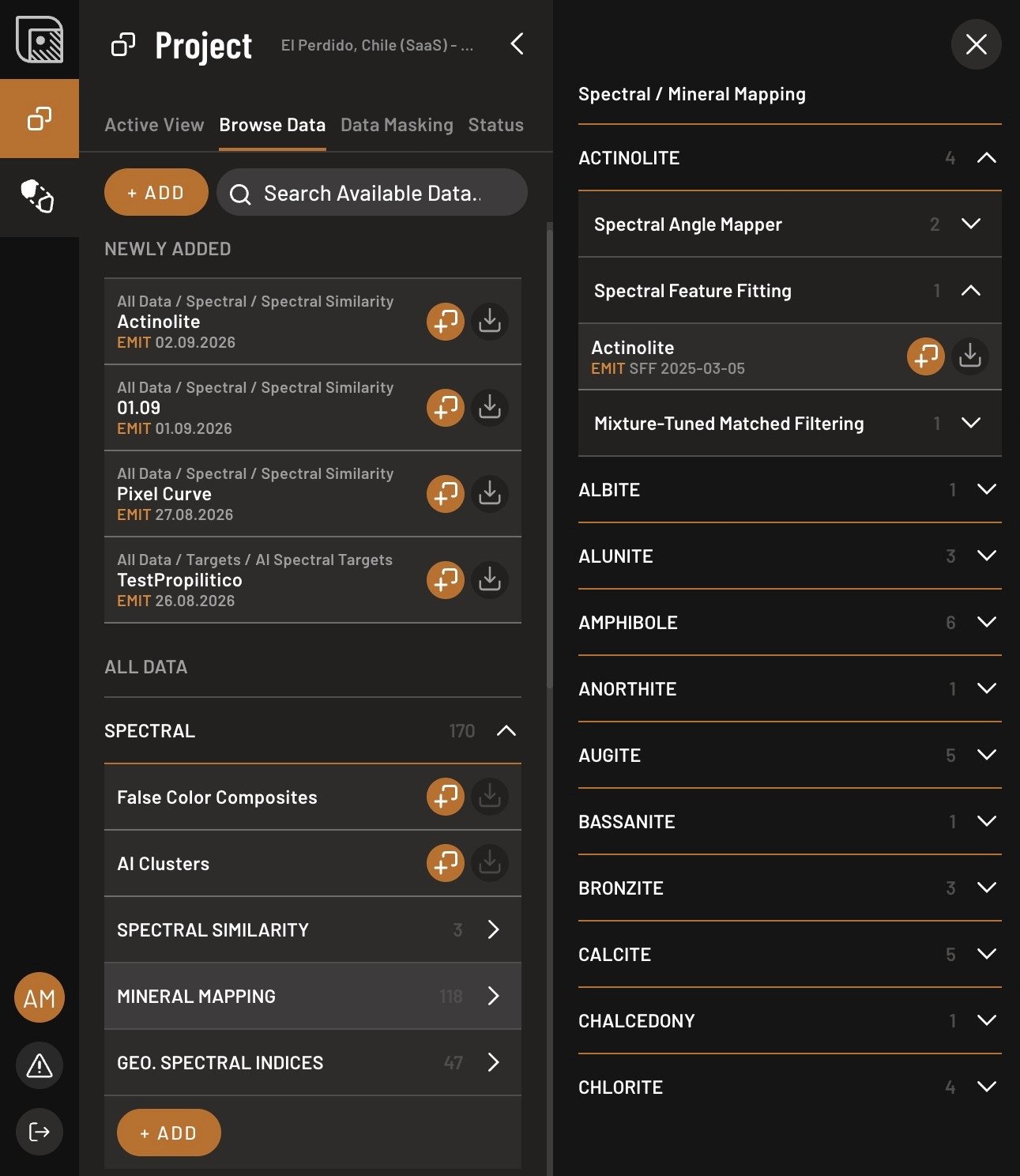
- Open Browse Data → Spectral → Mineral Mapping, pick a mineral, expand Spectral Feature Fitting and click Add layer.
- Drag the low end of the slider up until only the best-fitting pixels survive.
- Set the color, or switch to gradient mode, in the layer properties.
Give each mineral its own color. Where several overlap, that is the only way the map stays readable.
Where it misleads
Four failure modes survive a high threshold, and none of them looks wrong on the map:
- A different mineral in the same family. The most common outcome by a wide margin. Everything with Al-OH absorbs near 2200 nm: kaolinite, dickite, halloysite, illite, muscovite, montmorillonite, with pyrophyllite at about 2165 nm and alunite at about 2170 nm. Separating those means resolving the exact position and shape of the feature. A good fit confirms the family; the mineral needs more than the fit.
- A mineral that is not in the Spectral Library. SFF fits your ground to the references it has. Something absent gets fitted to whichever reference is nearest, and reports a respectable value for it.
- A surface coating. Lichen, desert varnish and dust sit between the sensor and the rock, and can produce features that fit cleanly.
- An atmospheric correction residual. A leftover from the correction step can mimic a real absorption, in the same place, across a whole scene.
The curve check catches the obvious failures, which is most of them, and none of these four. What catches them is comparing a pixel inside the zone against one outside it, knowing what your ground is covered in, and eventually a sample.