Analogy Lab
Every spectral method in the platform can return a false positive. The Analogy Lab is where you find out whether a particular pixel is one, by looking at the measurement instead of the map.
Two things make that comparison possible. Every spectral layer is atmospherically corrected to surface reflectance, which removes the atmosphere's own absorptions, and the library reference is resampled to your sensor's bands so that like is compared with like. Neither is perfect, and three consequences matter while you read a curve:
- The 1400 nm and 1900 nm regions are unusable. Atmospheric water vapor absorbs almost everything there, whatever the correction does. Whatever your curve appears to do in those gaps is not a mineral feature.
- Resampling is the bigger effect on a broad-band sensor. A library spectrum is measured at 1 to 2 nm. Convolved to Sentinel-2's bands, an entire 2200 nm absorption collapses into one 180 nm-wide channel.
- The correction does not normalize for slope or viewing geometry, and a library reference is a clean prepared powder while your pixel is weathered, coated and mixed at a different grain size. Both shift depths, which is why you read position rather than depth.
Inspect
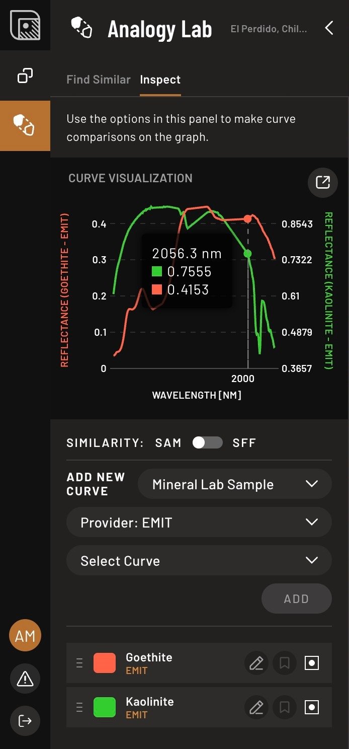
Click a pixel to plot its spectral curve. Then add a reference from the Spectral Library, or the reference spectrum behind a SAM or SFF result, so the two are drawn together. Plant curves are available alongside the mineral ones.
Read the dips, not the height. A real match has absorption features in the same places as the reference. Your curve will be shallower, because one pixel mixes rock, soil, dry vegetation and shadow, and that dilution is expected.
Read the size of the offset, too. A large offset means a different mineral. A small, systematic shift of a few nanometres is often the same mineral at a different composition: the white mica feature migrates from about 2195 to 2225 nm with Al content, and chlorite and carbonate features move with Fe/Mg ratio. Those shifts are used as proximity vectors toward a hydrothermal center, so a consistent small shift is worth mapping rather than dismissing as a failed match.
Then compare inside against outside. Plot a pixel from within your candidate zone and one from just outside it. If the two curves look the same, whatever you are seeing is not specific to the zone, and the result is probably not real.
Average, do not trust one pixel. SWIR signal-to-noise is low, so a shallow dip in a single unaveraged pixel can be noise. Take several pixels from inside the zone.
A rejection is the tool working. Note why it failed and move to the next candidate.
Curves worth recognizing
- The red edge. A sharp rise from about 700 nm, which green vegetation always has. Finding it in a pixel that survived masking means your vegetation mask is letting material through.
- Dry vegetation. The awkward one. It is not green, so a greenness index does not catch it, and its cellulose and lignin absorptions sit at about 2100 nm, immediately beside the 2200 nm clay feature, with more at about 1720 and 2300 nm. On Sentinel-2 one band covers both, so they cannot be separated at all.
- Snow. Bright across the visible, then dropping steadily through the near infrared to near-zero in the SWIR beyond about 1400 nm. How fast it drops depends on grain size, since old coarse snow darkens earlier than fresh. That SWIR collapse is how you separate it from bright soil.
What the curve check will not catch
- A different mineral in the same family. The commonest failure by a wide margin. Everything with Al-OH absorbs near 2200 nm — kaolinite, dickite, halloysite, illite, muscovite, montmorillonite — with pyrophyllite near 2165 and alunite near 2170 nm. The 2250 to 2350 nm region is shared by chlorite, epidote, talc, serpentine, calcite and dolomite. A curve that lines up confirms the family, not the mineral.
- A mineral you did not think to plot. Alunite against jarosite and gypsum, kaolinite against dickite, epidote against chlorite. The reference is in the library; it is just not on your screen.
- A mineral missing from the library. It gets fitted to whichever reference is nearest.
- A surface coating. Lichen, desert varnish and dust can produce features that line up cleanly.
- An atmospheric correction residual, which can mimic a real absorption across a whole scene.
Find Similar
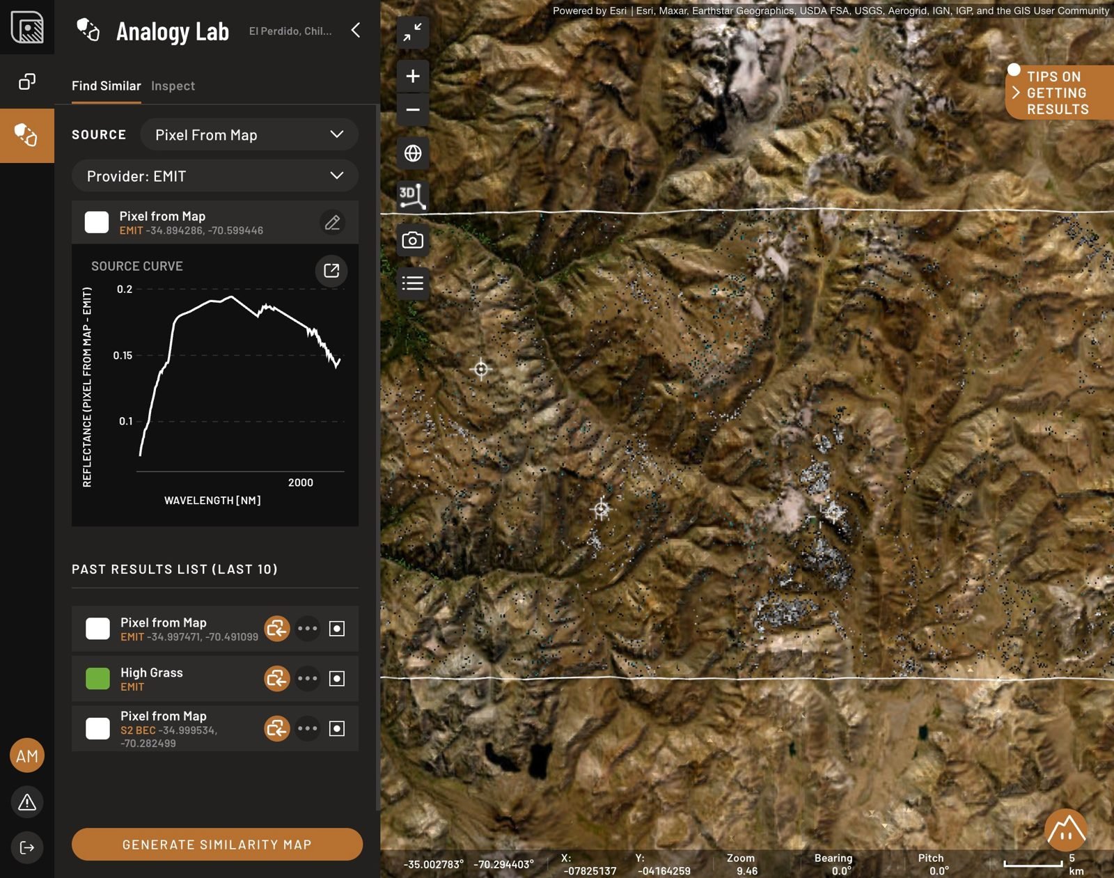
Give it a reference spectrum and it produces a similarity map, ranking every pixel in the area by how closely it resembles that spectrum.
The reference does not have to come from the area you are working in. A curve extracted from a pixel can be saved to the Spectral Library and then selected as the source in any project, so you can take a signature from ground you have mapped, sampled or drilled and search for analogues on ground you have not.
Used carefully that is powerful. Used carelessly it is the least reproducible operation in the platform, because a saved curve carries its own scene with it: that acquisition's atmospheric residual, sun and view geometry, season, soil moisture, vegetation background and regolith state. Matched into a different scene, those systematic differences can outweigh the mineralogy, and the similarity map will happily rank pixels on scene conditions rather than on rock.
Four conditions make a cross-area match worth something:
- The same sensor and the same processing chain. A signature saved from Sentinel-2's 12 bands means nothing against EMIT's 285, or the reverse.
- Comparable season and illumination.
- Comparable regolith and vegetation cover.
- A curve check in Inspect on every hit in the new area.
And note what transfers even when all four hold: a surface expression, not a deposit. Two areas can share a signature and only one of them have anything under it.